↜ Back to index Introduction to Numerical Analysis 1
Part a—Lecture 6
We continue looking at interesting ODE systems that are used in practice.
Lotka–Volterra equations
Let us consider a very simple model of two competing species, predator and prey, given by the Lotka-Volterra equations: \left\{ \begin{aligned} x' &= \alpha x - \beta x y,\\ y' &= \delta xy - \gamma y. \end{aligned} \right. Here x and y are the number of prey and predator, respectively, and \alpha, \beta, \gamma, \delta are positive real numbers describing the interaction of the species.
As a concrete example, consider rabbits as the prey and foxes as the predator species. If there are no foxes y = 0, rabbits multiply with rate \alpha. However, if there are foxes, some of the rabbits are eaten with rate \beta. Since foxes rely on rabbits for food, without rabbits (x = 0) the foxes will be dying off with rate \gamma. Catching rabbits allows foxes to multiply with rate \delta.
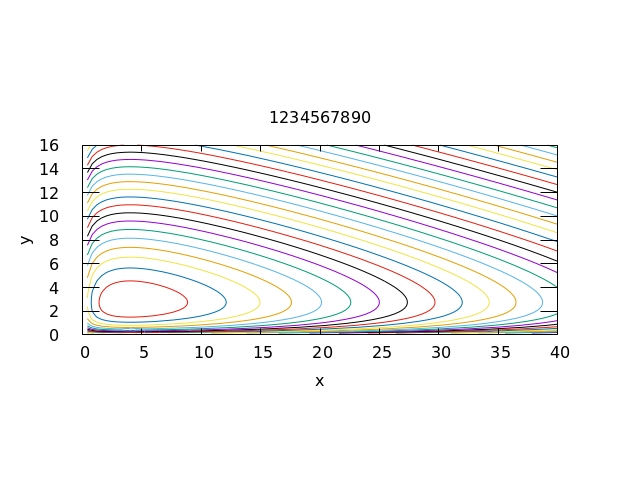
Exercise 1. While there is no explicit formula for the solution in general, consider the quantity \phi(x, y) := \delta x - \gamma \ln x + \beta y - \alpha \ln y, \qquad x, y > 0.
By computing the derivative using the chain rule, check that for any solution x(t), y(t) > 0 of the system the quantity \phi(x(t), y(t)) is constant.
Plot the contour plot of \phi using gnuplot with \alpha = 1.1, \beta = 0.4, \gamma = 0.4, \delta = 0.1. Use x range (0, 40) and y range for (0,16).
Submit the plot to LMS with your student ID as title.
Exercise 2.
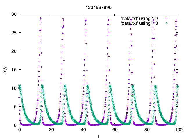
Write a Fortran program that solves the Lotka–Volterra equations using the midpoint method. In the following use, \alpha = 1.1, \beta = 0.4, \gamma = 0.4, \delta = 0.1 and h = 0.1.
Plot the solution x(t), y(t) as a function of t for initial data x(0) = 10, y(0) = 10 with t \in (0, 100).
Submit the plot to LMS with your student ID as the title.
Plot the parametric plot of the solution from 1.
Exercise 3.
Modify the program in Exercise 2 to print out the minimum of x and y and the maximum of x and y over the time interval t \in [0, 100]. Use the same parameters as in Exercise 2.
The program should print something like this:
$ ./a.exe
 Minimum of x and y:   2.22689882E-02  0.239500269
 Maximum of x and y:   28.8530903       10.7722187
Submit the program to LMS.
Example solutions to the exercises
1-1.

2-1.
